Scenery flow, conical densities, and rectifiability

January 9, 2015

Measure preserving flow

Ergodic theory studies the asymptotic behaviour of typical orbits of dynamical systems endowed with an invariant measure. Geometric measure theory can be described as a field of mathematics where geometric problems on sets and measures are studied via measure-theoretic techniques. Our main innovation is to apply the scenery flows to study classical problems in geometric measure theory which a priori do not involve any dynamics. The idea is to study the structure of a measure $\mu$ on $\mathbb{R}^d$ via dynamical properties of its magnifications at a given point $x \in \mathbb{R}^d$. Rather than individual results, we believe that our main contribution is to highlight the relevance of ergodic-theoretic methods around the scenery flow in geometric problems. Let $X$ be a metric space and write $\mathbb{R}_+ = [0,\infty)$. A one-sided flow is a family $(S_t)_{t \in \mathbb{R}_+}$ of maps $S_t \colon X \to X$ for which

$$S_{t+t'} = S_{t} \circ S_{t'}, \qquad t,t' \in \mathbb{R}_+.$$

In other words, $(S_t)$ is an additive $\mathbb{R}_+$ action on $X$. If $(X,\mathcal{B},P)$ is a probability space, then we say that $P$ is $S_t$ invariant if $S_t P = P$ for all $t \geq 0$. In this case, we call $(X,\mathcal{B},P,(S_t)_{t \in \mathbb{R}_+})$ a measure preserving flow. A set $A \in \mathcal{B}$ is $S_t$ invariant if $P(S_t^{-1} A \triangle A)=0$. A measure preserving flow is ergodic, if for all $t \geq 0$ the measure $P$ is ergodic with respect to the transformation $S_t \colon X \to X$, that is, for all $S_t$ invariant sets $A \in \mathcal{B}$ we have $P(A) \in \{ 0,1 \}$.

Theorem 1 (Birkhoff ergodic theorem). If $(X,\mathcal{B},P,(S_t)_{t \in \mathbb{R}_+})$ is an ergodic measure preserving flow, then for a $P$ integrable function $f \colon X \to \mathbb{R}$ we have

$$\lim_{T \to \infty} \frac{1}{T} \int_0^T f(S_t x) \,\mathrm{d} t = \int f \,\mathrm{d} P$$

at $P$ almost every $x \in X$.

Theorem 2 (Ergodic decomposition). Any $S_t$ invariant measure $P$ can be decomposed into ergodic components $P_\omega$, $\omega \sim P$, such that

$$P = \int P_\omega \,\mathrm{d} P(\omega).$$

Ergodic decomposition is unique up to $P$-measure zero sets.

Scenery flow

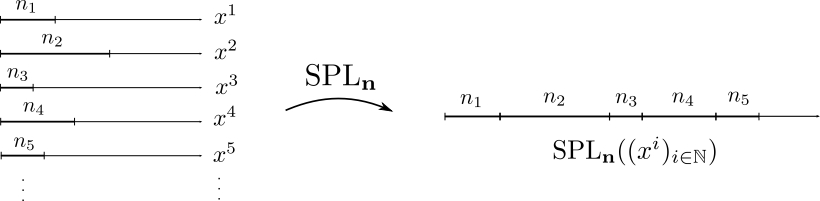
Let $\mathcal{M}_1 = \mathcal{P}(B_1)$ be the collection of all Borel probability measures on the unit ball $B_1$ and $\mathcal{M}_1^* = \{ \mu \in \mathcal{M}_1 : 0 \in \mathrm{spt}\mu \}$. Define the magnification $S_t\mu$ of $\mu \in \mathcal{M}_1^*$ at $0$ by

$$S_t\mu(A) = \frac{\mu(e^{-t}A)}{\mu(B(0,e^{-t}))}, \qquad A \subset B_1.$$

Due to the exponential scaling, $(S_t)_{t \in \mathbb{R}_+}$ is a flow in the space $\mathcal{M}_1^*$ and we call it the scenery flow at $0$. Although the action $S_t$ is discontinuous (at measures $\mu$ with $\mu(\partial B_1) > 0$) and the space $\mathcal{M}_1^* \subset \mathcal{M}_1$ is not closed (but it is Borel), the scenery flow behaves in a very similar way to a continuous flow on a compact metric space. If we have a Radon measure $\mu$ and $x \in \mathrm{spt}\mu$, we want to consider the scaling dynamics when magnifying around $x$. Let $T_x\mu(A) = \mu(A+x)$ and define $\mu_{x,t} = S_t(T_x\mu)$. Then the one-parameter family $(\mu_{x,t})_{t \in \mathbb{R}_+}$ is called the scenery flow at $x$. Accumulation points of this scenery in $\mathcal{M}_1$ will be called tangent measures of $\mu$ at $x$ and the family of tangent measures of $\mu$ at $x$ is denoted by $\mathrm{Tan}(\mu,x) \subset \mathcal{M}_1$. We are not interested in a single tangent measure, but the whole statistics of the scenery $\mu_{x,t}$ as $t \to \infty$, i.e. the tangent distribution. The tangent distribution of $\mu$ at $x \in \mathrm{spt}\mu$ is any weak limit of

$$\langle \mu \rangle_{x,T} = \frac{1}{T} \int_0^T \delta_{\mu_{x,t}} \,\mathrm{d} t.$$

The family of tangent distributions of $\mu$ at $x$ is denoted by $\mathcal{TD}(\mu,x) \subset \mathcal{P}(\mathcal{M}_1)$. The integration above makes sense since we are on a convex subset of a topological linear space. We emphasize that tangent distributions are measures on measures. If the limit above is unique, then, intuitively, it means that the collection of views $\mu_{x,t}$ will have well defined statistics when zooming into smaller and smaller neighbourhoods of $x$. Notice that the set $\mathcal{TD}(\mu,x)$ is non-empty and compact at $x \in \mathrm{spt}\mu$. Moreover, the support of each $P \in \mathcal{TD}(\mu,x)$ is contained in $\mathrm{Tan}(\mu,x)$.

Fractal distributions

We say that the distribution $P$ on $\mathcal{M}_1$ is scale invariant if it is $S_t$ invariant, that is, $S_tP = P$ for all $t \ge 0$, and quasi-Palm if for any Borel set $\mathcal{A} \subset \mathcal{M}_1$ with $P(\mathcal{A}) = 1$ it holds that $P$ almost every $\nu \in \mathcal{A}$ satisfies

$$\nu_{z,t} \in \mathcal{A}$$

for $\nu$ almost every $z \in \mathbb{R}^d$ with $B(z,e^{-t}) \subset B_1$. Roughly speaking, the quasi-Palm property guarantees that the null sets of the distributions are invariant under translations to a typical point of the measure. The distribution $P$ on $\mathcal{M}_1$ is a fractal distribution (FD) if it is scale invariant and quasi-Palm. A fractal distribution is an ergodic fractal distribution (EFD) if it is ergodic with respect to $S_t$. Write $\mathcal{FD}$ and $\mathcal{EFD}$ for the set of all fractal distributions and ergodic fractal distributions, respectively. A general principle is that tangent objects enjoy some kind of spatial invariance. For example, Preiss (1987) proved that tangent measures to tangent measures are tangent measures. For tangent distributions, a very powerful formulation of this principle is the following theorem.

Theorem 3 (Hochman (2010+)). For any Radon measure $\mu$ and $\mu$ almost every $x$, all tangent distributions at $x \in \mathrm{spt}\mu$ are fractal distributions.

Notice that as the action $S_t$ is discontinuous, even the scale invariance of tangent distributions or the fact that they are supported on $\mathcal{M}_1^*$ are not immediate, though they are perhaps expected. The most interesting part in the above theorem is that a typical tangent distribution satisfies the quasi-Palm property. Hochman’s result is highly nontrivial. It is proved by using CP processes which are Markov processes on the dyadic scaling sceneries of a measure introduced by Furstenberg. Technical difficulties of the proof include an interplay between fractal distributions and CP processes, restricted and extended versions of distributions, and different norms. Although fractal distributions are defined in terms of seemingly strong geometric properties, the family of fractal distributions is in fact very robust.

Theorem 4 (K-Sahlsten-Shmerkin (2015)). The family of fractal distributions is compact.

The result may appear rather surprising since the scenery flow is not continuous, its support is not closed, and, more significantly, the quasi-Palm property is not a closed property. The proof of this result is also based on the interplay between fractal distributions and CP processes, and restricted and extended versions of distributions. Together with convexity, the theorem implies that the family of fractal distributions is in fact a Choquet simplex.

Theorem 5 (K-Sahlsten-Shmerkin (2015)). The family of fractal distributions is a Poulsen simplex, i.e. a Choquet simplex in which extremal points are dense.

Note that the set of extremal points is precisely the collection of ergodic fractal distributions. The proof of this result is again based on the interplay between fractal distributions and CP processes. We prove that ergodic CP processes are dense by constructing a dense set of distributions of random self-similar measures on the dyadic grid. This is done by first approximating a given CP process by a finite convex combination of ergodic CP processes, and then, by splicing together those finite ergodic CP processes, constructing a sequence of ergodic CP processes converging to the convex combination. Roughly speaking, splicing of measures consists in pasting together a sequence of measures along dyadic scales. Splicing is often employed to construct measures with a given property based on properties of the component measures.

This idea was used in the movie Splice in 2009 where scientists formed new species by splicing together DNA of different animals. Schmeling-Shmerkin (2010) used the idea to investigate the dimensions of iterated sums of Cantor sets and Hochman (2010+) employed it to construct certain examples.

Uniformly scaling measures

In geometric considerations, we usually construct a fractal distribution satisfying certain property. We often want to transfer that property back to a measure. This leads us to the concept of generated distributions. We say that a measure $\mu$ generates a distribution $P$ at $x$ if

$$\mathcal{TD}(\mu,x) = \{ P \}.$$

Furthermore, $\mu$ is a uniformly scaling measure (USM) if $\mu$ generates $P$ at $\mu$ almost every $x$. One can think that uniformly scaling property is an ergodic-theoretical notion of self-similarity. Hochman (2010+) proved the striking fact that generated distributions are always fractal distributions. The following result is a converse to this.

Theorem 6 (K-Sahlsten-Shmerkin (2015)). For any fractal distribution $P$, there exists a uniformly scaling measure $\mu$ generating $P$.

By the compactness and the Poulsen property (by the Birkhoff ergodic theorem, the claim holds for ergodic fractal distributions), it suffices to show that the collection of fractal distributions satisfying the claim is closed. The proof of this is again based on the interplay between fractal distributions and CP processes. Even though the previous theorem concerns measures which have a single tangent distribution at typical points, perhaps surprisingly, it gives us an application which shows that the exact opposite holds for a Baire generic measure.

Theorem 7 (K-Sahlsten-Shmerkin (2015)). For a Baire generic Radon measure $\mu$, the set of tangent distributions is the set of all fractal distributions at $\mu$ almost every $x$.

The result continues the work of O’Neil (1994) and Sahlsten (2014) who proved that a Baire generic measure has all Borel measures as tangent measures at almost every point.

Dimension of fractal distributions

Intuitively, the local dimensions of a measure should not be affected by the geometry of the measure on a density zero set of scales. Thus one could expect that tangent distributions should encode all information on dimensions.

Theorem 8 (Hochman (2010+)). If $P$ is a fractal distribution, then $P$ almost every measure is exact dimensional. Furthermore, if $P$ is ergodic, then the value of the dimension is $P$ almost everywhere constant.

The dimension of a fractal distribution $P$ is

$$\dim P = \int \dim\mu \,\mathrm{d} P(\mu).$$

It is straightforward to see that the function $P \mapsto \dim P$ defined on the family of fractal distributions is continuous.

Theorem 9 (Hochman (2010+)). For any Radon measure $\mu$ and for $\mu$ almost every $x$, the pointwise dimensions satisfy

$$\begin{align*} \overline{\dim}_{\mathrm{loc}}(\mu,x) &= \sup\{ \dim P : P \in \mathcal{TD}(\mu,x) \text{ is a fractal distribution} \}, \\ \underline{\dim}_{\mathrm{loc}}(\mu,x) &= \inf\{ \dim P : P \in \mathcal{TD}(\mu,x) \text{ is a fractal distribution} \}. \end{align*}$$

In particular, if $\mu$ is a USM generating a fractal distribution $P$, then $\mu$ is exact dimensional and $\dim\mu = \dim P$.

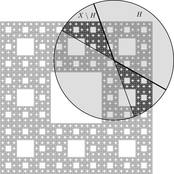
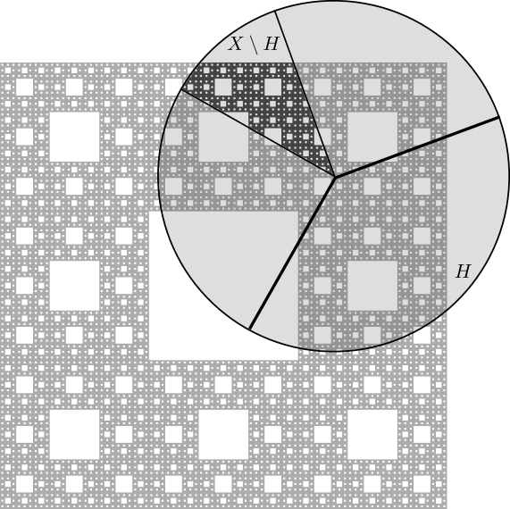
Conical densities and rectifiability

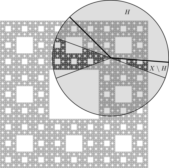
Let $G(d,d-k)$ denotes the space of all $(d-k)$-dimensional linear subspaces of $\mathbb{R}^d$ and set $S^{d-1} = \{ x \in \mathbb{R}^d : |x|=1 \}$. For $x \in \mathbb{R}^d$, $r>0$, $V \in G(d,d-k)$, $\theta \in S^{d-1}$, and $0<\alpha\le 1$ define

$$\begin{align*} X(x,r,V,\alpha) &= \{ y \in B(x,r) : \mathrm{dist}(y-x,V) < \alpha|y-x| \}, \\ H(x,\theta,\alpha) &= \{ y \in \mathbb{R}^d : (y-x) \cdot \theta \ge \alpha|y-x| \}. \end{align*}$$

For example, the set $X(x,r,V,\alpha) \setminus H(x,\theta,\alpha)$ when $d=3$ and $k=1$ is as follows:

Conical density results aim to give conditions on a measure (for example, a lower bound on some dimension) which guarantee that the non-symmetric cones $X(x,r,V,\alpha) \setminus H(x,\theta,\alpha)$ contain a large portion of the mass from the surrounding ball $B(x,r)$ for certain proportion of scales.

Theorem 10 (K-Sahlsten-Shmerkin (2015)). If $d \in \mathbb{N}$, $k \in \{ 1,\ldots,d-1 \}$, $k < s \le d$, and $0 < \alpha \le 1$, then there exists $0 < \varepsilon < \varepsilon(d,k,\alpha)$ satisfying the following: For every Radon measure $\mu$ on $\mathbb{R}^d$ with $\underline{\dim}_{\mathrm{H}} \mu \ge s$ it holds that

$$\liminf_{T \to \infty} \frac{1}{T} \,\mathcal{L}^1\Bigl(\Bigl\{ t \in [0,T] : \inf_{\genfrac{}{}{0pt}{}{\theta \in S^{d-1}}{V \in G(d,d-k)}} \frac{\mu(X(x,e^{-t},V,\alpha) \setminus H(x,\theta,\alpha))}{ \mu(B(x,e^{-t}))} > \varepsilon \Bigr\}\Bigr) \ge \frac{s-k}{d-k}$$

at $\mu$ almost every $x \in \mathbb{R}^d$. If the measure $\mu$ only satisfies $\underline{\dim}_{\mathrm{p}}\mu \ge s$, then the above inequality holds with $\limsup_{T \to \infty}$ at $\mu$ almost every $x \in \mathbb{R}^d$.

         

Tangent distributions are well suited to address problems concerning conical densities. The cones in question do not change under magnification and this allows to pass information between the original measure and its tangent distributions. The inequality in Theorem 10 can be restated as

$$\liminf_{T \to \infty} \langle \mu \rangle_{x,T}(\mathcal{B}_\varepsilon) \ge \frac{s-k}{d-k},$$

where

$$\mathcal{B}_\varepsilon = \bigl\{ \nu \in \mathcal{M}_1 : \inf_{\genfrac{}{}{0pt}{}{\theta \in S^{d-1}}{V \in G(d,d-k)}} \nu(X(0,1,V,\alpha) \setminus H(0,\theta,\alpha)) > \varepsilon \bigl\}.$$

This is the main link between the geometric problem we consider and the scenery flow. Recalling Theorem 6, we let $\mu$ be the uniformly scaling measure generating

$$P = \frac{s-k}{d-k} \delta_\mathcal{L} + \Bigl( 1-\frac{s-k}{d-k} \Bigr) \delta_\mathcal{H},$$

where $\mathcal{L}$ is the normalization of $\mathcal{L}^d|_{B_1}$ and $\mathcal{H}$ is the normalization of $\mathcal{H}^k|_{W \cap B_1}$ for a fixed $W \in G(d,k)$. By Theorem 8, the Radon measure $\mu$ is of exact dimension $s$ and it can be shown that the limit $\lim_{T \to \infty} \langle \mu \rangle_{x,T}(\mathcal{B}_\varepsilon)$ exists and equals $\frac{s-k}{d-k}$ for all small enough $\varepsilon > 0$. Therefore, the inequality in Theorem 10 can be considered sharp.

The proof of Theorem 10 is based on showing that there cannot be “too many” rectifiable tangent measures. This means that, perhaps surprisingly, most of the known conical density results are, in some sense, a manifestation of rectifiability. A set $E \subset \mathbb{R}^d$ is called $k$-rectifiable if there are countably many Lipschitz maps $f_i \colon \mathbb{R}^k \to \mathbb{R}^d$ so that

$$\mathcal{H}^k\Bigl( E \setminus \bigcup_i f_i(\mathbb{R}^k) \Bigr) = 0.$$

Moreover, we say that a Radon measure $\nu$ is $k$-rectifiable if $\nu \ll \mathcal{H}^k$ and there exists a $k$-rectifiable set $E\subset\mathbb{R}^d$ such that $\nu(\mathbb{R}^d\setminus E)=0$. A set $E \subset \mathbb{R}^d$ is called strongly $k$-rectifiable if there exist countably many Lipschitz maps $f_i \colon \mathbb{R}^k \to \mathbb{R}^d$ so that

$$E \subset \bigcup_i f_i(\mathbb{R}^k).$$

A Radon measure $\mu$ is purely $k$-unrectifiable if it gives no mass to $k$-rectifiable sets and $E$ is purely $k$-unrectifiable if the restriction $\mathcal{H}^k|_E$ is purely $k$-unrectifiable. A strongly $k$-rectifiable set is obviously $k$-rectifiable. Any set $E \subset \mathbb{R}^d$ with $\mathcal{H}^k(E) = 0$ and $\dim_{\mathrm{p}}(E)>k$ is $k$-rectifiable but not strongly $k$-rectifiable. Furthermore, it follows from analyst’s traveling salesman theorem that any set of upper Minkowski dimension strictly less than $1$ is strongly $1$-rectifiable.

About the proof

Let us sketch the proof of Theorem 10. For each $0<\alpha\le 1$, defining a closed set $\mathcal{A}_\varepsilon = \mathcal{M}_1 \setminus \mathcal{B}_\varepsilon$, i.e.

$$\mathcal{A}_\varepsilon = \bigl\{ \nu \in \mathcal{M}_1 : \nu(X(0,1,V,\alpha) \setminus H(0,\theta,\alpha)) \le \varepsilon \text{ for some } V \in G(d,d-k) \text{ and } \theta \in S^{d-1} \bigl\},$$

the task is to show that there exists a small enough $\varepsilon > 0$ such that every Radon measure $\mu$ on $\mathbb{R}^d$ with $\underline{\dim}_{\mathrm{H}} \mu \ge s$ satisfies $\limsup_{T \to \infty} \langle \mu \rangle_{x,T}(\mathcal{A}_\varepsilon) \le 1 - \frac{s-k}{d-k}$ at $\mu$ almost every $x \in \mathbb{R}^d$. The proof of Theorem 10 is basically just the machinery of fractal distributions and the following rectifiability criterion.

Lemma 11. A set $E \subset \mathbb{R}^d$ is strongly $k$-rectifiable if for every $x \in E$ there are $V \in G(d,d-k)$, $\theta \in S^{d-1}$, $0 < \alpha < 1,$ and $r > 0$ so that $E \cap X(x,r,V,\alpha) \setminus H(x,\theta,\alpha) = \emptyset$.

Let $0 < p < \frac{s-k}{d-k}$. Suppose to the contrary that there is $0<\alpha\le 1$ so that for each small enough $\varepsilon > 0$ there exists a Radon measure $\mu$ with $\underline{\dim}_{\mathrm{H}}\mu \ge s$ such that

$$\limsup_{T \to \infty}\,\langle \mu \rangle_{x,T}(\mathcal{A}_\varepsilon) > 1-p,$$

on a set $E_\varepsilon$ of positive $\mu$ measure. Fix $\delta>0$ such that $p < \frac{s-\delta-k}{d-k}$. Relying on Theorem 3 and Theorem 9, we may assume that all tangent distributions of $\mu$ at points $x \in E_{\varepsilon}$ are fractal distributions, and

$$\inf\{\dim P : P \in \mathcal{TD}(\mu,x)\} = \underline{\dim}_{\mathrm{loc}}(\mu,x) > s-\delta.$$

Fix $x \in E_{\varepsilon}$. For each small enough $\varepsilon > 0$, as $\mathcal{A}_\varepsilon$ is closed, we find a tangent distribution $P_{\varepsilon} \in \mathcal{TD}(\mu,x)$ so that $P_{\varepsilon}(\mathcal{A}_\varepsilon) \ge 1-p$. Since the sets $\mathcal{A}_\varepsilon$ are nested and closed, we see that

$$P(\mathcal{A}_0) = \lim_{\varepsilon \downarrow 0} P(\mathcal{A}_\varepsilon) \ge 1-p,$$

where $P$ is a weak$^*$ limit of a sequence formed by $P_\varepsilon$ as $\varepsilon \downarrow 0$. Furthermore, since the collection of all fractal distributions is closed by Theorem 4 and the dimension is continuous, the limit distribution $P$ is a fractal distribution with

$$\dim P \ge s-\delta.$$

Recalling Theorem 2, let

$$P = \int P_\omega \,\mathrm{d} P(\omega)$$

be the ergodic decomposition of $P$. By the invariance of $\mathcal{A}_0$, we have $P_\omega(\mathcal{A}_0) \in \{0,1\}$ for $P$ almost all $\omega$. If $P_\omega(\mathcal{A}_0) = 0$, we use the trivial estimate

$$\dim P_\omega \le d.$$

If $P_\omega(\mathcal{A}_0) = 1$, then, using the quasi-Palm property, for $P_\omega$ almost every $\nu$ and for $\nu$ almost every $z$ the normalized translation $\nu_{z,t_z}$ is an element of $\mathcal{A}_0$ for some $t_z > 0$ with $B(z,e^{-t_z}) \subset B_1$. For each such $\nu$ let

$$E = \{ z \in B_1 : \nu_{z,t_z} \in \mathcal{A}_0 \}$$

be this set of full $\nu$ measure. Thus for every $z \in E$ there are $V \in G(d,d-k)$ and $\theta \in S^{d-1}$ with

$$E \cap X(z,e^{-t_z},V,\alpha) \setminus H(z,\theta,\alpha) = \emptyset.$$

Lemma 11 implies that $E$ is strongly $k$-rectifiable. In particular, $\dim \nu \le k$, which yields $\dim P_\omega \le k$. Since $P(\{ \omega : P_\omega(\mathcal{A}_0) = 1 \}) = P(\mathcal{A}_0) \ge 1-p$ we estimate

$$s-\delta \leq \dim P = \int \dim P_\omega \,\mathrm{d} P(\omega) \leq P(\mathcal{A}_0)k + (1-P(\mathcal{A}_0))d \le (1-p)k + pd$$

which gives $p \ge \frac{s-\delta-k}{d-k}$. But this contradicts the choice of $\delta$.

Average unrectifiability

Pure unrectifiability is also a condition which guarantees that the measure is scattered in many directions. We introduce average unrectifiability and show that it implies a conical density result. Under certain assumption, we also show the converse. Given a proportion $0 \leq p < 1$, we say that a Radon measure $\mu$ is $p$-average $k$-unrectifiable if we have

$$P(\{\nu \in \mathcal{M}_1 : \mathrm{spt}\nu \text{ is not strongly } k \text{-rectifiable}\}) > p$$

for every $P \in \mathcal{TD}(\mu,x)$ at $\mu$ almost every $x$.

Theorem 12 (K-Sahlsten-Shmerkin (2015)). Suppose that $d \in \mathbb{N}$, $k \in \{ 1,\ldots,d-1 \}$, and $0 \le p < 1$. If $\mu$ is $p$-average $k$-unrectifiable, then for every $0 < \alpha \le 1$ there exists $0 < \varepsilon < 1$ so that

$$\liminf_{T \to \infty} \frac{1}{T} \langle \mu \rangle_{x,T}(\mathcal{B}_\varepsilon) > p$$

at $\mu$ almost every $x \in \mathbb{R}^d$.

Since, by Theorem 10, the critical dimension for conical densities around $k$-planes is precisely $k$, it is perhaps natural to try to prove the converse for measures of this dimension.

Theorem 13 (K-Sahlsten-Shmerkin (2015)). Suppose that $d \in \mathbb{N}$, $k \in \{ 1,\ldots,d-1 \}$, $0 \le p < 1$, $0<\alpha,\varepsilon<1$, and a Radon measure $\mu$ satisfies

$$0 < \liminf_{r \downarrow 0} \frac{\mu(B(x,r))}{r^k} \leq \limsup_{r \downarrow 0} \frac{\mu(B(x,r))}{r^k} < \infty$$

and

$$\liminf_{T \to \infty} \frac{1}{T} \langle \mu \rangle_{x,T}(\mathcal{B}_\varepsilon) > p$$

at $\mu$ almost all $x \in \mathbb{R}^d$. Then for $\mu$ is $p$-average $k$-unrectifiable.